Modelling community uniqueness with `gdmmTMB`
modelling_community_uniqueness.RmdAlthough the response variable in a Generalised Dissimilarity Model
(GDM) is a pairwise dissimilarity, gdmmTMB can also handle
effects on community uniqueness that are mathematically equivalent to
those in models where uniqueness metrics, such as the Local Contribution
to Beta Diversity (LCBD), are the response.
This vignette showcases the usage of gdmmTMB to model
community uniqueness using the dataset microbialdata
available as part of the gllvm R package. The dataset
contains the matrices Y, with abundances of over 900
species found across 56 microbial communities, and Xenv,
which consists of multiple environmental variables measured at each
site
Xenv <- gllvm::microbialdata$Xenv
Y <- gllvm::microbialdata$Y
For the purpose of this example, we focus on pH as the
main driver of community variability.
Modelling linear effects on community uniqueness
Community uniqueness is often modelled as the Local Contribution to Beta Diversity (Legendre and De Cáceres 2013). A common approach is to (1) compute LCBD scores from a dissimilarity matrix and (2) model LCBD scores as independent observations.
The code below computes LCBD scores using the package
adespatial (Dray et al.
2018), and regresses them against pH and the quadratic pH
term.
LCBD <- adespatial::LCBD.comp(vegan::vegdist(Y))
Xenv$LCBD <- LCBD$LCBD

m_lcbd <- lm(LCBD~poly(pH,2), data = Xenv)
Xenv$pred_lcbd <- predict(m_lcbd)

ggplot(Xenv , aes(x = pH, y = LCBD)) +
  geom_point() +
  geom_line(aes(y = pred_lcbd)) +
  theme(aspect.ratio = 1)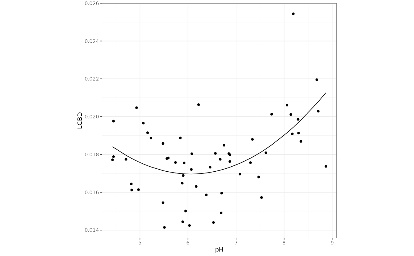
In brief, effects on LCBD denote increasing or decreasing expected dissimilarities of each community to all other communities. The U-shaped relationship above therefore indicates that communities at the extremes of the pH gradient are more dissimilar on average to all other communities, and therefore more unique.
We can obtain the exact same relationship by modelling pairwise
dissimilarities directly, by introducing site-level effects (see Hernández-Carrasco et al. (2025) for details).
This can be done in gdmmTMB via the
uniq_formula argument:
# fit model
m_gdmm <-
  gdmm(Y = Y,
       X = Xenv,
       uniq_formula = ~ poly(pH, 2))
#> Warning: the 'nobars' function has moved to the reformulas package. Please
#> update your imports, or ask an upstream package maintainer to do so.

# generate predictions
Xenv$pred_gdmm <- predict(m_gdmm, component = 'uniqueness', scale_uniq = TRUE, CI = F)

# Plot relationship
ggplot(Xenv , aes(x = pH, y = LCBD)) +
  geom_point() +
  geom_line(aes(y = pred_gdmm, col = 'gdmm'), linewidth = 2, alpha = 0.7) +
  geom_line(aes(y = pred_lcbd, col = 'lcbd')) +
  theme(aspect.ratio = 1,
        legend.position = 'bottom')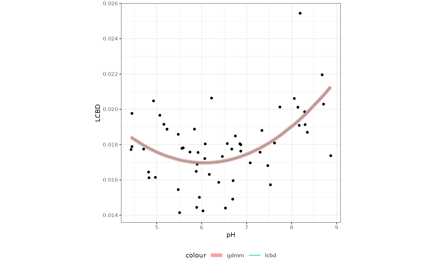
Both models produce the exact same U-shaped relationship between
pH and LCBD. However, modelling effects on
uniqueness with pairwise dissimilarities allows accounting for the
distribution of such dissimilarities with a more appropriate error
distribution and link function. For instance, a binomial error
distribution can be specified via the family argument. We
can also account for the non-independence of pairwise dissimilarities
with a site-level random effect
(uniq_formula = ~ ... + (1|site)), or with Bayesian
bootstrapping (bboot = TRUE):
Xenv$site <- as.factor(1:nrow(Xenv))

# site-level random effect
m_gdmm2 <- gdmm(
  Y = Y,
  X = Xenv,
  uniq_formula = ~ poly(pH, 2) + (1 | site),
  family = 'binomial')

# Bayesian bootstrapping
m_gdmm3 <- gdmm(
  Y = Y,
  X = Xenv,
  uniq_formula = ~ poly(pH, 2),
  family = 'binomial',
  bboot = TRUE)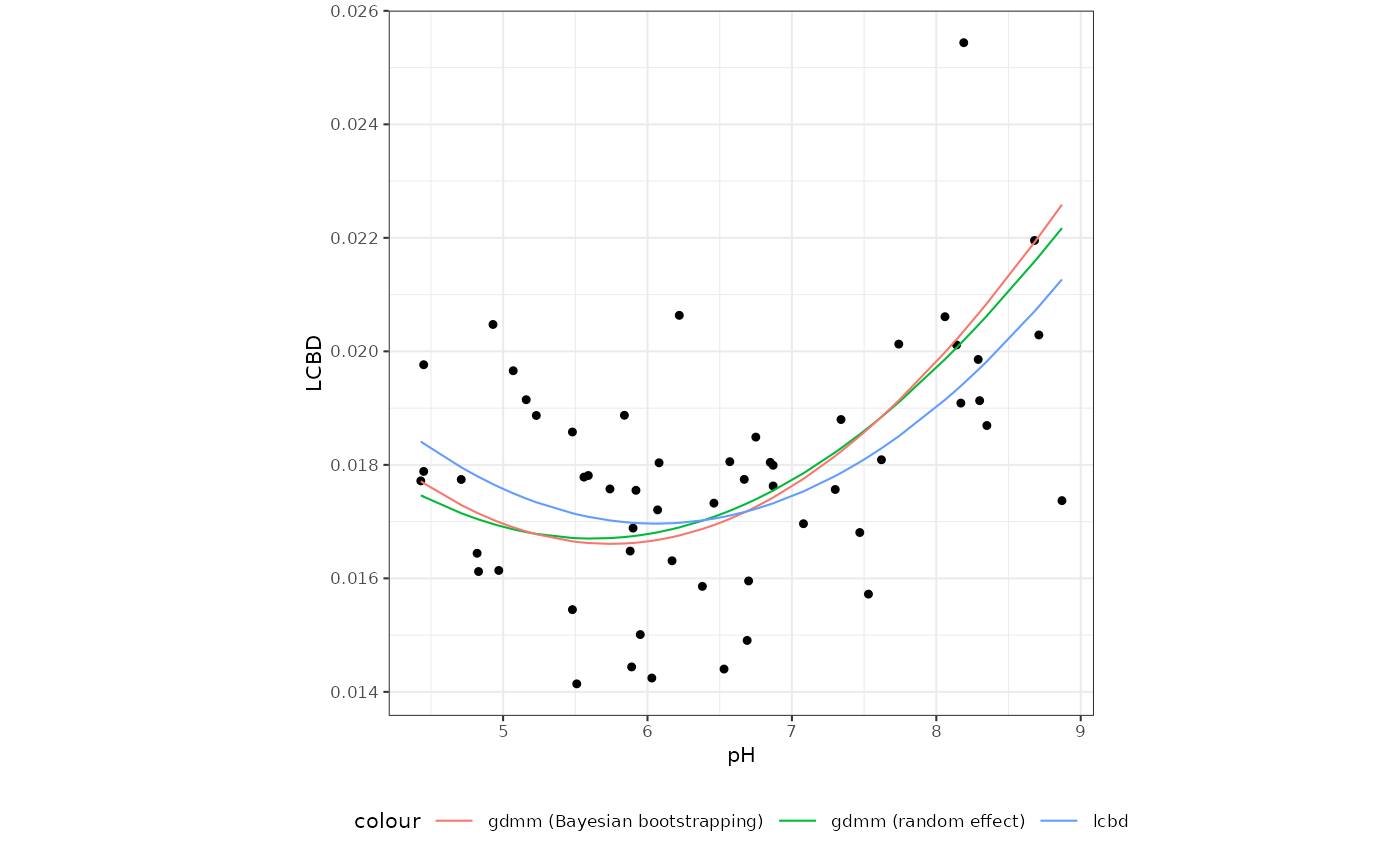
Accounting for directional community changes
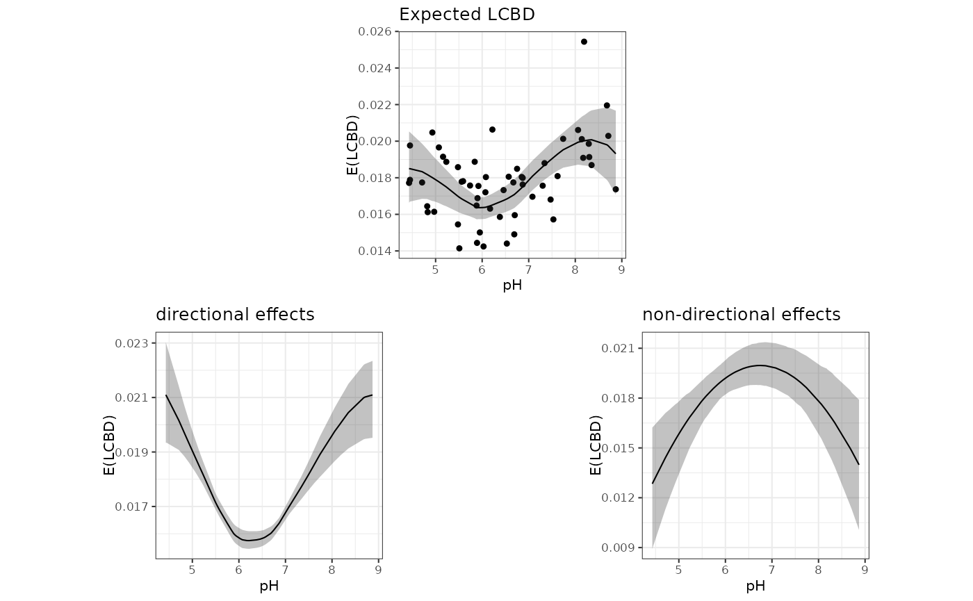
The U-shaped relationship between LCBD and pH above indicates that sites with low and high pH host relatively more unique species. However, a representation of the variability in community composition reveals a strong directional change in community composition along the pH gradient.
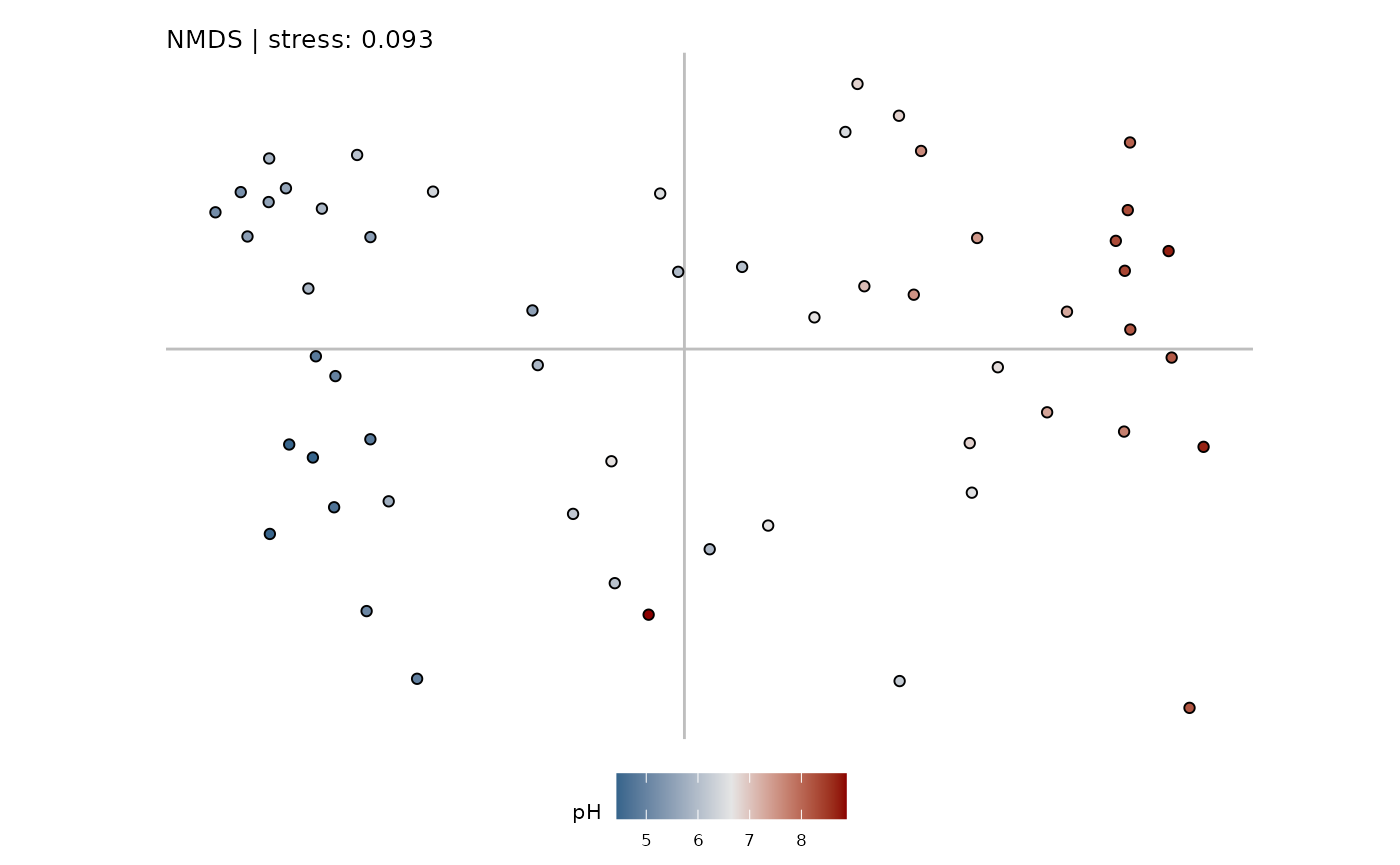
Sites at either end of the pH gradient are therefore further from the
centroid (i.e., they present a higher average dissimilarity to all other
sites), which could underpin the U-shaped relationship between LCBD and
pH. We refer to the contribution of directional changes in community
composition to the observed beta diversity patterns as ‘directional
effects’. Directional effects can be accounted for by making the
expected dissimilarity between sites a function of their environmental
distance (Mokany et al. 2022). In
gdmmTMB, these directional effects are introduced via the
diss_formula argument:
m_gdmm3 <- gdmm(
  Y = Y,
  X = Xenv,
  uniq_formula = ~ poly(pH, 2),
  diss_formula = ~ isp(pH),
  family = 'binomial',
  bboot = TRUE,
  mono = TRUE)
The diss_gradient function can be used to visualise
dissimilarity gradients.
diss_grad <- diss_gradient(m_gdmm3)

ggplot(do.call(rbind, diss_grad), aes(x = x, y = f_x))  +
  geom_line() +
  geom_ribbon(aes(ymin = `CI 2.5%`, ymax = `CI 97.5%`), alpha = 0.3) +
  xlab('pH') +
  ylab('f(pH)')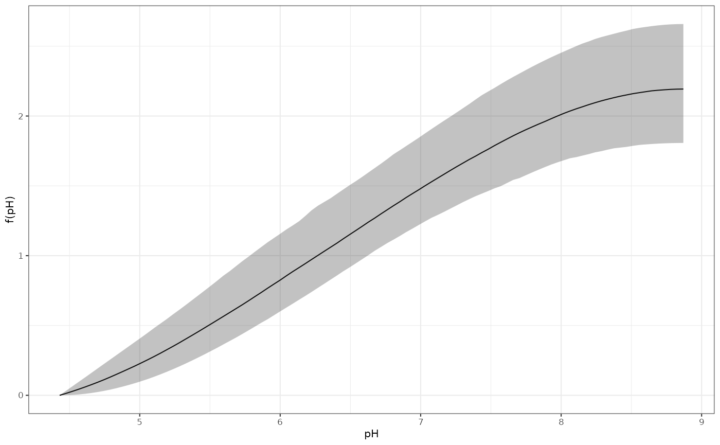
We can also use the predict method to visualise the new
expected relationship between pH and LCBD, and the contributions of each
model component (directional and non-directional effects):
newdata_mean = data.frame(pH = rep(mean(Xenv$pH), nrow(Xenv)))

predict_tot <- data.frame(
  predict(m_gdmm3, new_X = Xenv, new_W = Xenv, component = 'uniqueness'),
  pH = Xenv$pH,
  LCBD = Xenv$LCBD)

predict_dir <- data.frame(
  predict(m_gdmm3, new_X = Xenv, new_W = newdata_mean, component = 'uniqueness'),
  pH = Xenv$pH,
  LCBD = Xenv$LCBD)

predict_nondir <- data.frame(
  predict(m_gdmm3, new_X = newdata_mean, new_W = Xenv, component = 'uniqueness'),
  pH = Xenv$pH,
  LCBD = Xenv$LCBD)